Accuracy of small-sample interpolated empirical distribution functions: a simulation
Accuracy of small-sample interpolated empirical distribution functions: a simulation When you have a few data points, and no model of the distribution they are drawn from, you can still use what you have to estimate how that distribution behaves. For example, you may wonder what’s a 95th percentile of that distribution is.
There are several approaches for going from the data you have to a distribution that (hopefully) approximates the true distribution they were drawn from well:
Using some parametric model (i.e assuming they are drawn from some known distribution like Normal, Gamma, mixtures of these, …) and a method of estimating the model parameters from the data (MLE, etc.) Using some non-parametric estimation procedure [1]. The method I analyze here is the one that linearly interpolates between your data points, which is the default when you use numpy.percentile() in python or quantile(type=4) in R [2] How does it look like? Say you only have two samples: You intercepted two spies and their ages were 19 and 33. You’d like to know what the probability a spy is 28 years old is, or you want to know what the 95th percentile of spy ages are, but you only have these two spies. The classical empirical CDF from these two would assume:
(a) There is 0% chance of a spy being under 19 years old.
(b) There is 0% chance of a spy being over 33 years old.
(c) The distribution has two point masses at 19 and 33, so all percentiles between 0 and 50 are 19 and all percentiles between 50-100 are 33, and there’s essentially zero probability of having a spy aged between 20 and 30 for instance.
This sounds like an unnatural assumption, but it’s odd to use an empirical CDF with two points in practise. Empirical CDFs are really useful in proofs where there are $latex n$ samples and $latex n \rightarrow \infty$. It helps show that they converge to the true distribution, they cleanly manage discrete/discontinuities in distributions, and they converge fast, and in many cases are easy to show how the rate of convergence behaves (asymptotics).
But in scenarios where you actually want to use a few data points to generate some other information about the likely distribution, a simple yet practical assumption is using a linearly interpolated CDF. This would assume:
(a) There is 0% chance of a spy being under 19 years old.
(b) There is 0% chance a spy is over 33 years old.
(c) All percentiles between 0% and 100% map to ages distributed uniformly between 19 and 33 - i.e the 50th percentile is a spy being 26 years old, and the interquartile range (25th-75th percentiles) are that a spy is between 22.5 and 29.5 years old.
If you had 4 points, you essentially assume the first is the 0th percentile of the distribution, the second is the 33rd percentile, the third is the 66th percentile and the last is the 100th (maximum value); The rest of the percentiles are interpolated in a piecewise-linear manner between each two points. For example, this chart shows a random, uniform draw of 4 points from $latex [0,1]$, the resulting interpolated CDF (in red), the original CDF of the Uniform[0,1] distribution (blue), and the resulting error in estimating each of the percentiles.
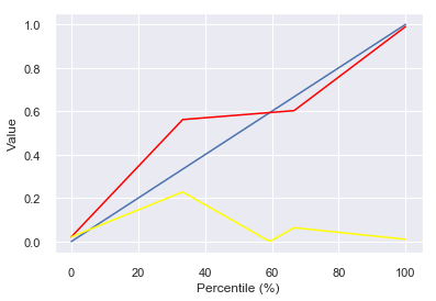
My random draw of four points from $latex [0,1]$ was [0.98980661, 0.02112006, 0.5617029 , 0.60289351]. As it happened to have two points quite close to the ends of the range $latex [0,1]$ (.989 and .021), it approximates most of the range pretty well, with the maximal error being around percentile 30: Because the empirical distribution assumes the 33th percentile is .561 while in truth it is .33, the maximal error of is around $latex .561-.33=.23$.
You now understand what small-sample, linearly interpolated empirical CDFs are! Let’s assess their accuracy, using simulations.
Accuracy of small-sample interpolated ECDFs This leads us to estimating the error. In another draw I would’ve had $latex \frac{1}{2^3} = \frac{1}{8}$ chance of having all 4 points randomly generated from the distribution be under 0.5 or have all 4 of them be over 0.5. In these cases, the maximal error would be more than 0.5 (eg, if all four are under 0.5, my 100th percentile would be less than 0.5 whereas the real 100th percentile of Uniform[0,1] is 1). What should we use as the “error” function summarising how far an interpolated ECDF using a draw of $latex N$ samples is from some distribution? And how does that error distribute (so, how likely we are when drawing $latex N$ samples to get an error of X? How does that change with $latex N$, or with the (unknown) distribution we’ve drawn from?). We’re going to answer all of these questions next.
There are as always many options for a choice of summarizing error but two natural ones arise that I focus on:
(Approximate) $latex L_{\infty}$: This is asking what the maximal error is: What’s the percentile of the original distribution that our distribution is furthest from. The problem with calculating this in a simulation is that many distributions are unbounded - i.e there’s some chance they’ll generate arbitrarily high (or low negative) numbers. However, our interpolated ECDF always has a clear minimum and maximum value: The lowest and highest sample - these are its 0th and 100th percentile, where for an unbounded distribution one of these or both will be infinity (or minus infinity), so the $latex L_{\infty}$ as I define it would be infinite. So instead, I just measure, for bins of 1% width, what is the maximal distance between the value of the original CDF for that percentile, and our simulated interpolated ones - essentially the ‘maximum’ value of the yellow line in the chart above. This is similar to the Kolmogorov-Smirnov statistic for ECDFs, but is easier for me to calculate for this interpolated CDF in practice. (approximate) $latex L_{1}$ : This averages the distances between the CDF and the approximate CDF. It captures more information about the range of errors, at the loss of info about how great the error is maximally.
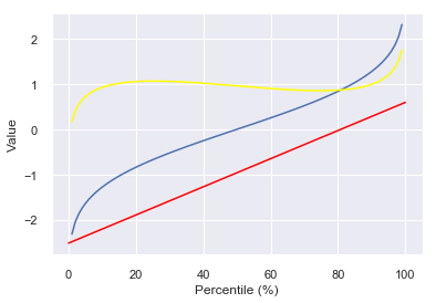
Two draws from the Standard Normal distribution gave me [~-2.5, ~0.5]. The $latex L_{\infty}$ here is the 99th percentile, where the difference is almost 2. The $latex L_{1}$ is ~1, because on average the error is close to 1.
Simulations The theory of Empirical CDFs promises some pretty quick convergence in many cases for the original (not interpolated) method. But how does it behave in practise in low-sample scenarios? Below are charts with the mean $latex L_{\infty}$ (blue lines), mean L_1 (red lines) and standard deviation of the $latex L_{\infty}$ (grey line) for simulations drawing 2-30 samples from the Normal, Exponential(1), Poisson(1), Beta(2,2), Gamma(2,2) and Uniform(0,1) distributions. The notebook that does this is here, so you can easily generate ones for your own distribution.
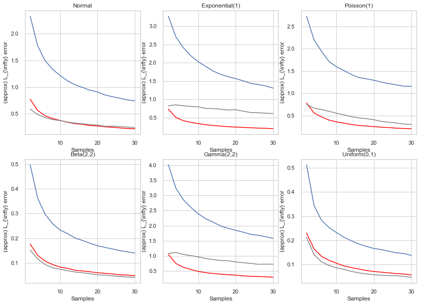
I also recommend for practical cases, if you had 30 samples, to just randomly choose e.g 5 of these every time and see how well they approximate the CDF you approximate with 30 points, to give you a sense of how the scale of the error looks (and perhaps fitting that line try and project from 30 onwards). But regardless some rules of thumb emerge - the maximal error in estimating percentiles 1-99 drops from an average of 2-3 times the variance of the distribution with 2 samples to ~1 times the variance or just under that for 30 samples.
Footnotes [1] For instance, the Empirical CDF is the standard way to treat this mathematically, and Kernel Density Estimation is a better, but more complicated method that also requires some tuning.